When we have a dataset on hand, it is often of our interest to run a quick analysis and get some insights. The analysis usually includes making predictions of a new dataset, grouping records, identifying important features, and optimization. We can achieve these goals by building a machine learning model and use the trained model to make predictions, cluster analysis, feature important analysis, and optimization. All of these can be easily done with the 012_DOE_DataAnalyzer workflow available for all users. There are four components of this workflow.
- Learn and Predict
- Feature Importance
- Optimization
- Cluster Analysis
Each component will generate a report that contains a summary of the analysis results.

Learn and Predict
On d3VIEW, there are an abundance of machine learning models available for users to explore. An easy way for choosing the model is to select multiple of them and d3VIEW will automatically choose the model that has the best performance. Here is a list of available ML models
- Linear Regression
- Lasso Regression
- Ridge Regression
- SVR Regression
- Random Forest Regression
- Gradient Boost Regression
- Decision-Tree Regression
- GPR Regression
- MLP Regression
- Elasticnet Regression
- Bayesian Ridge Regression
The Learning process will build the model and generate plots to compare the true values and predicted values for each target feature using the first two input features selected.
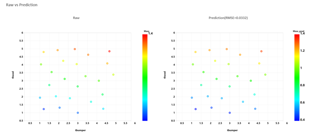
Prediction process will show the predicted values against the reference values provided by users. If no prediction dataset is provided, the output will be the same as the learning report.
Feature Importance with SOBOL
Feature Importance
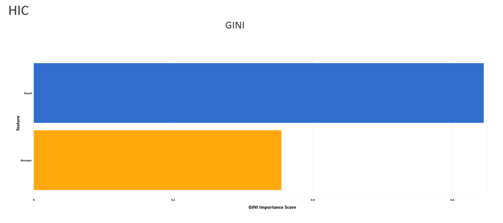
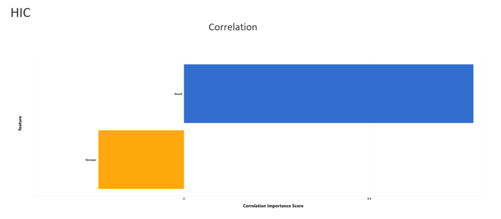
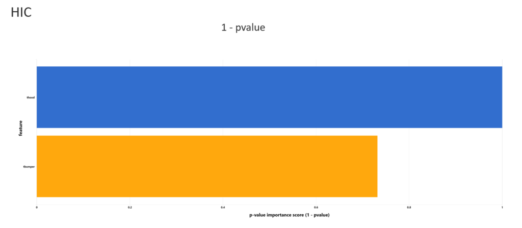
Feature importance analyzes the relationship between input features and target features and rank them by GINI importance scores. Top 5 features will be shown, together with the other metrics such as correlation and p-value scores (1-p-value).
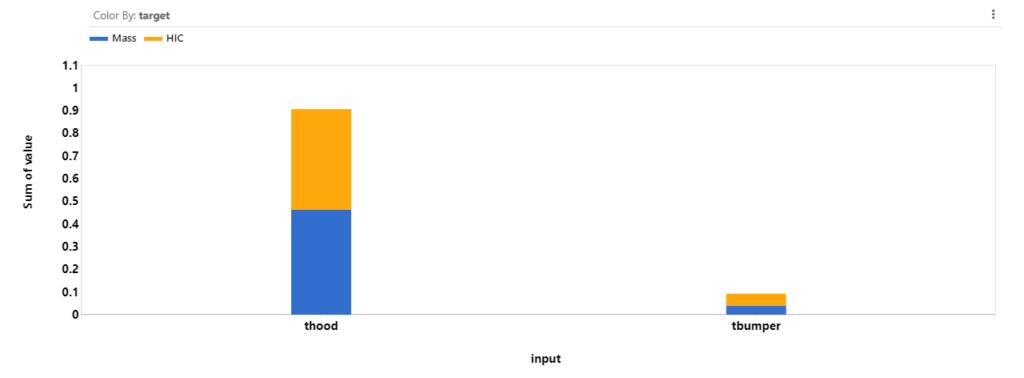
Global Sensitivity Analysis with Sobol
Feature importance report also include a sobol plot for sensitivity analysis. This provides another perspective on the input feature influence on the targets.
Optimization
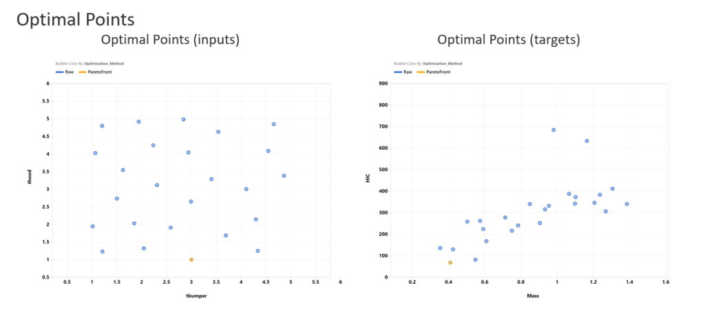
Optimization process uses Pareto Front Optimization method to find the point that is closest to the ideal point. User can specify the target value for each target feature. The optimal point will be the point that is “closest” to the specified target point.
Cluster Analysis
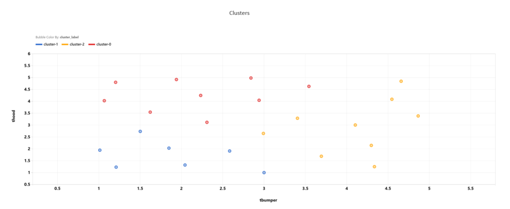
Cluster Analysis component groups points to specified groups using input features, target features or both. In the report, a scatter plot using the first two input features specified by users is colored by clusters.
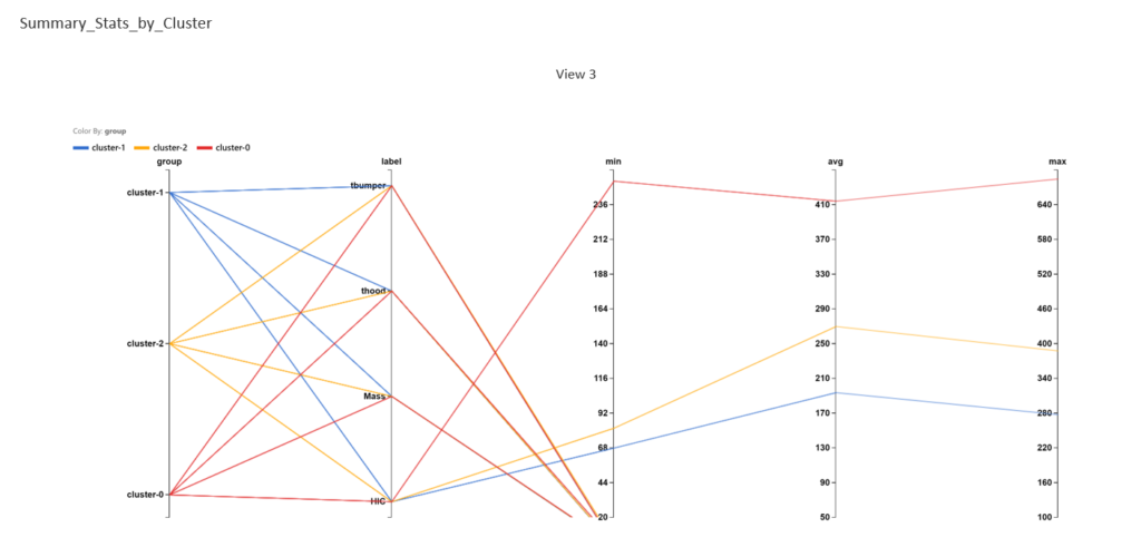
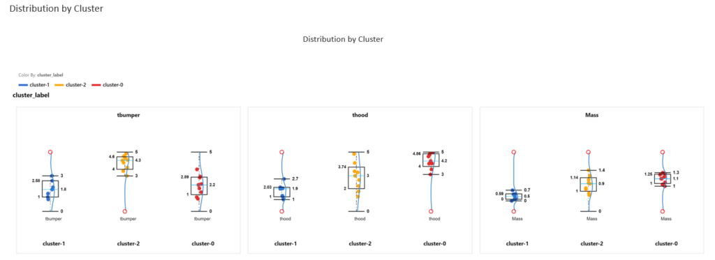
Statistics from each cluster is also listed to provide more information on the characteristics for each cluster.
Distribution plots provide an insight for each variable in different clusters.
Workflow Execution
To execute the workflow, click “AutoPlay” to start. Then we are prompted to choose the task we want to perform. For each task, we may have different settings we need to configure. For example, Cluster Analysis requires an input for the number of clusters, and what features we want to use for clustering.
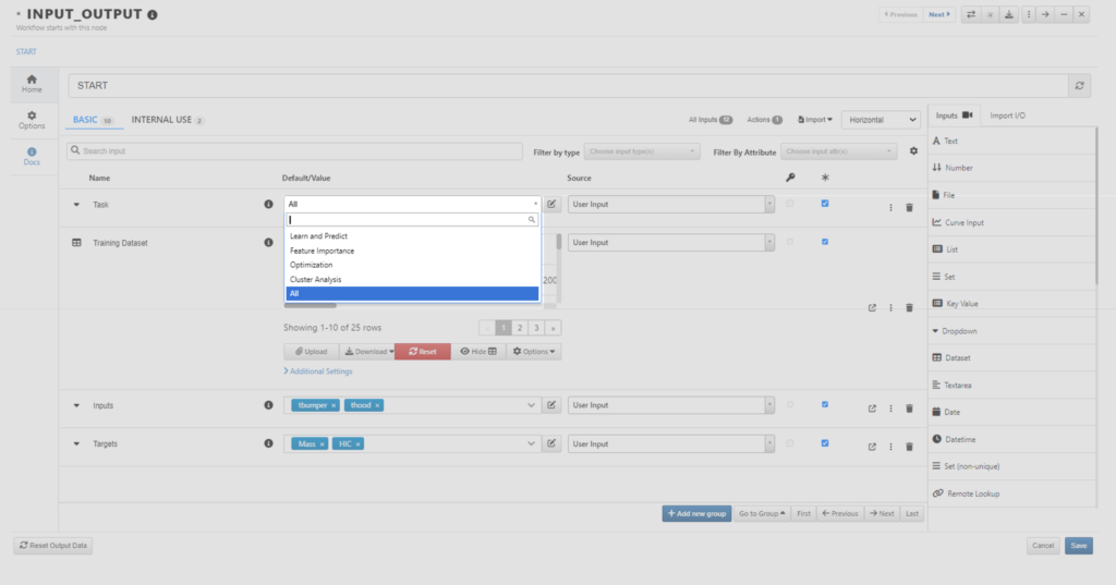
The common inputs are input dataset that we want to analyze, input features and target features.

After the configuration is complete, we can continue to execute the workflow. When the execution is complete, we can click to open the Reporter worker and view the reports.
Generate Sampling Points
doe_sampling_point_generator worker generates new sampling points based on the conditions provided in the input dataset using selected sampling mechanism. The dataset includes the name, variable type (continuous, constant, or discrete), min and max (for continuous variables), and discreteValues (for discrete variables). We can choose the number of experiments (number of rows in the output dataset) using the “number of experiments” option. Points per variables determines the possible values (for continuous variables) to sample from. The values will be evenly distributed in the variable domain (defined by min and max).
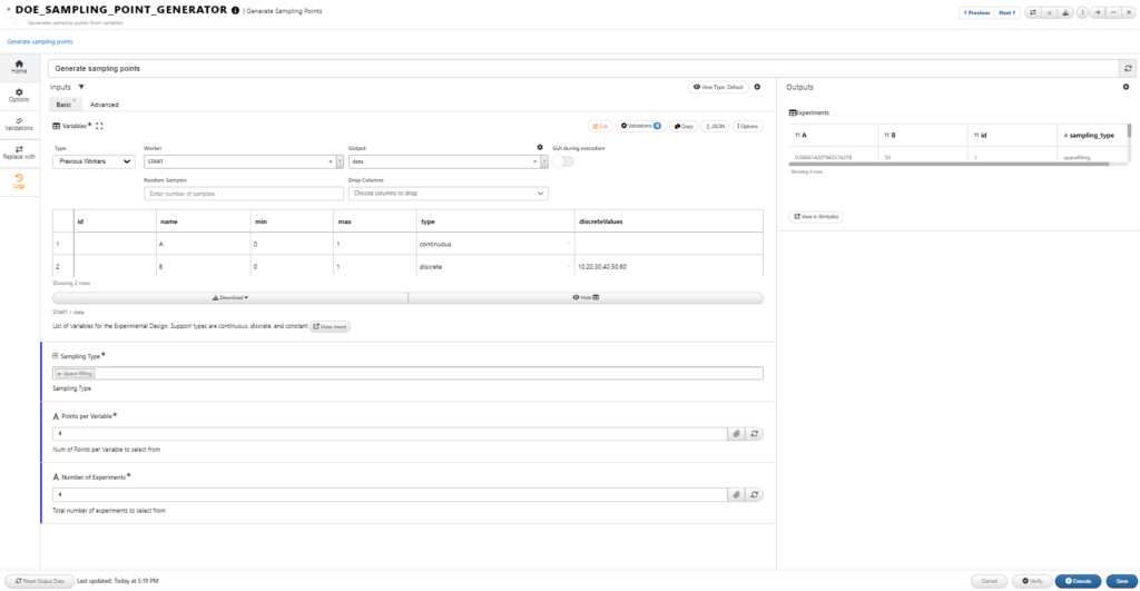
There are a few options for selecting sampling points. Each has their own advantages and disadvantages. Overall, Full Factorial exploits all possible combinations of values. It can be computationally expensive when the number of variables are large. D Optimal points tend to concentrate at the corners of the design space. LHS and Space Filling result tend to scatter more evenly in the design space.

When we have a discrete variable, the output will only include specified values from the “discreteValues” column from the input dataset.


