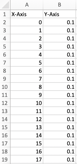
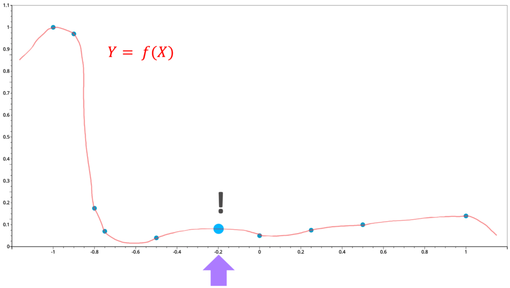
It is not unusual that due to various limitations, researchers can only collect limited number of samples. Meanwhile, for many analyses, we desire a higher resolution. In two-dimension case, we have X and Y coordinates of our points. We are interested in what happens in between any of the two points.
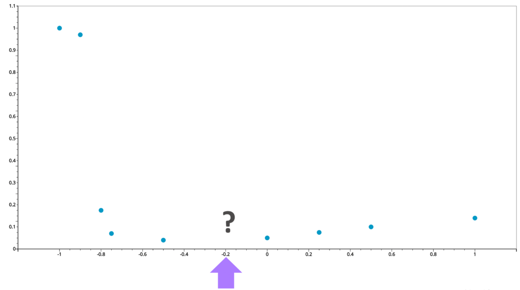
We can draw a curve passing through these points to describe the relationship between X and Y values. With such a curve at hand, we can estimate the unobserved values in between any observed points. From this perspective, we consider interpolation as a procedure of looking for a function to describe the relationship between X and Y and using this function to estimate the values at any location.
Linear interpolation
Linear interpolation is the most straightforward and commonly used interpolation method. It comes naturally when we have two points, we connect them with a straight line to fill out the missing information in between. By doing so, we made our assumption that the points on the line represent the unobserved values. When there are more than two points, we simply connect any pair of adjacent points with straight lines. This is piecewise interpolation in the sense that on each subinterval formed by two adjacent points, we use a different line segment to represent the missing values. It is possible that all the points lie on the same line, but we still go through the procedure of connecting every individual pair of points.
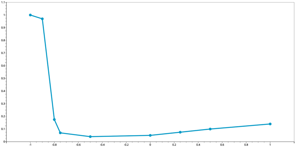
Linear interpolation works the best when we have many points. When there are more points, drastic change in values of two adjacent points is less likely. Imagine the route from work to home. We can use one point to represent the workplace and one for home. When we connect them and claim that’s our way home, we are missing a lot of details. If we take a point for every mile, we get more details. But we may still miss a U-turn. Instead, if we take a point every 10 yards, our route is much less likely to miss anything major like a U-turn (even when we do miss, the error is much less) and any two adjacent points will have more similar values. Some discrepancies in between any two adjacent points are small and thus can be ignored. This is also why the linear interpolation is the default method for visualizing discrete data points.
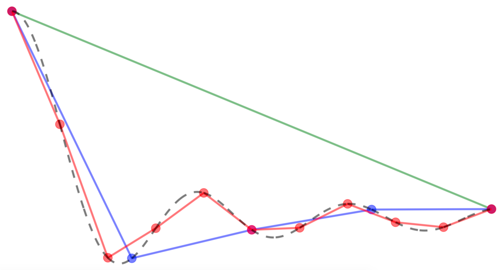
When we have fewer points, the pursuit for higher accuracy prevails. And the errors between the interpolated values and their true values have a larger impact on the analysis. Thus, more interpolation methods are created in order to meet such demands. One of the examples is polynomial interpolation.
Polynomial interpolation
Polynomial interpolation assumes that the points are samples taken from a polynomial curve. We know that a straight line can be described by a linear function, which is a special case of polynomial of degree 1 and that a parabola can be described by a quadratic function, which is a polynomial of degree 2. We also know that any two points determines a line. Meanwhile we can describe three or more points by a linear function if all these points lie on the same line. Hence, N points can be described by a polynomial of no more than N-1 degrees. Consequently, there must exist a polynomial with the least number of degrees that describes all the points. This polynomial, given the observed points, is called a Lagrange polynomial.
Piecewise cubic hermite interpolation
Generally, when we speak of linear interpolation, we mean piecewise linear interpolation. We don’t find a linear function to describe all points. Rather, we find one linear function on each subinterval formed by two adjacent points, and thus “piecewise”. It provides more flexibility for the variations between different subintervals. We can do the same for polynomial interpolation. And the most effective methods developed use cubic polynomials for each subinterval (i.e., polynomials of degree 3). Since at least four points are required to uniquely determine a cubic polynomial, in order to have a unique solution, we need to add more constraints. And these constraints are the slopes at each point.
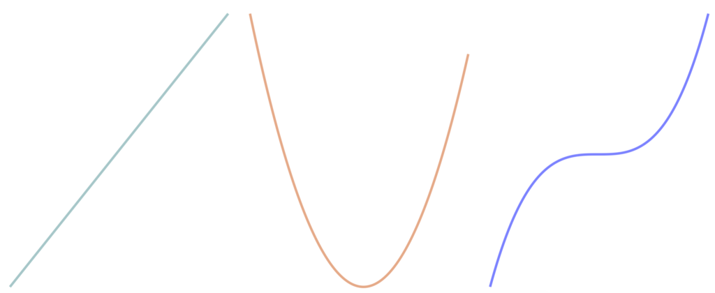
It is noticeable that, if no consecutive three points lie on one line, the slopes of two line segments formed by any consecutive three points have different slopes. This causes a sharp corner at each point. The slope at each point of a line is the same across the line. But this is not the case for functions of higher orders nor for piecewise functions. In order to describe their “slopes” at each point, we take the derivatives of the function at each point which is essentially the “slope” at that point. The corner at each point can be explained by the jump at that point due to the different values of their derivatives on the left and on the right.
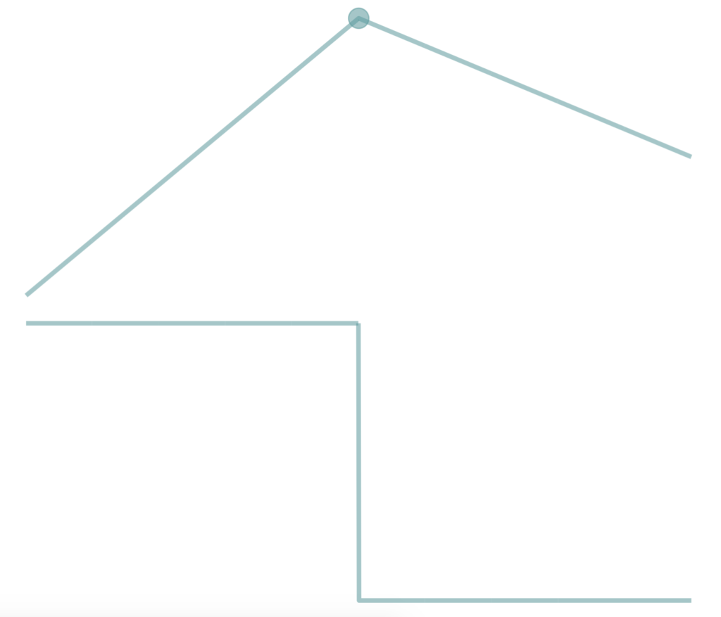
A line is the only option for linear interpolation on each subinterval, there is nothing we can do about these corners. For piecewise polynomial interpolation, it is possible to find two cubic polynomials on the left and right of a point such that they have the same slope at that point. The final piecewise polynomial constructed in such manner shows a smoother look. We can go further from here. Not only we want slopes of the interpolation polynomial at each point equal from left and right, but also the slopes of the derivative function (first derivative) and their derivative functions (second, third, … derivatives). Some people claim all polynomials that passes through all give points are Hermite interpolation polynomials without any requirements for their derivative functions. Here we say, polynomials that pass through all points and at least have a continuous first derivative function (thus no jump in slopes and no corners at every point) are called Hermite interpolation polynomials.
Pchip, cubic spline, makima
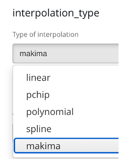
Piecewise Cubic Hermite Interpolation Polynomials are abbreviated as “pchip”. Many softwares exclusively refer to interpolation polynomials that only have a continuous first derivative function as pchip. And if we require an additional continuous second derivative function, then it becomes a cubic spline. The difference between these two methods is how the derivatives at the points are defined. And there are other ways to definite it too and one of them is makima.
Compare interpolation outputs on d3VIEW
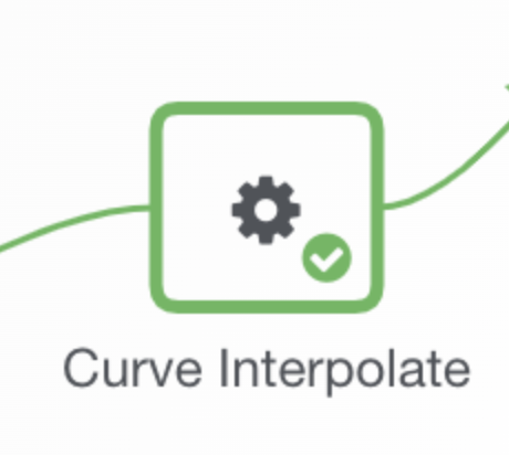
On d3IVEW, we have fully integrated these interpolation methods to a worker that we can add to a workflow. We can choose which method to apply and on what X values to interpolate. Instead of typing all the values manually, we can also provide an expression in the format of “start_value:end_value:increment_step”.


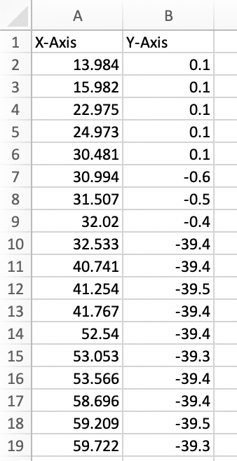
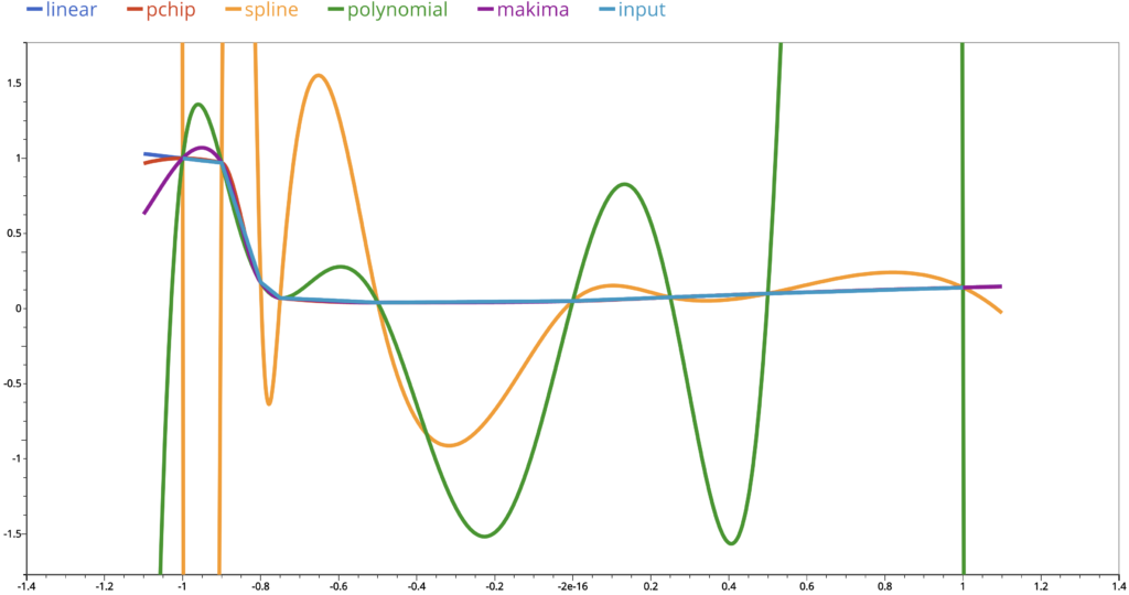
Now we will use the following example to demonstrate the interpolation methods we have talked about so far and compare their results.
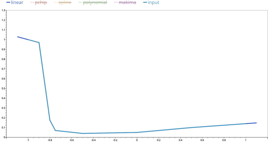
When we connect the dots, we get the output from linear interpolation. As we discussed above, the visualization of input points is an implement of linear interpolation. We should not be surprised that they are the same.
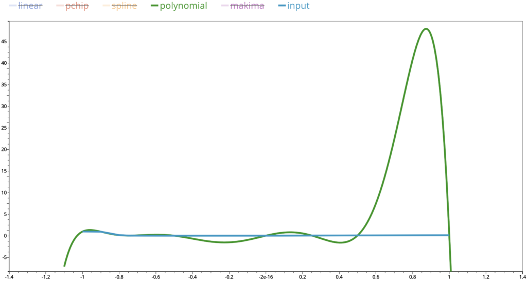
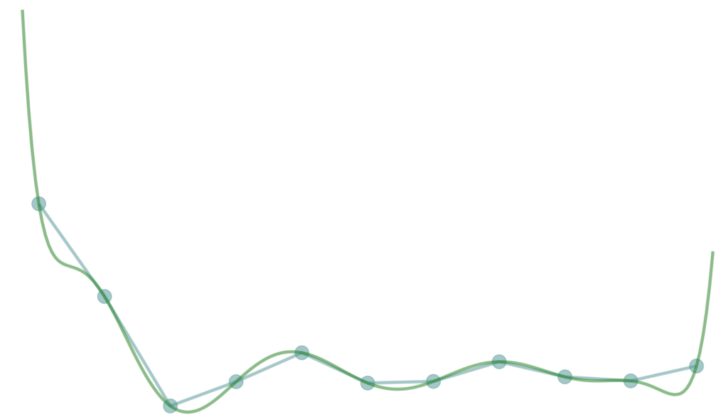
This is the output from polynomial interpolation. We can see that at the right end, there is a huge difference in the interpolated values compared to those of the linear one.
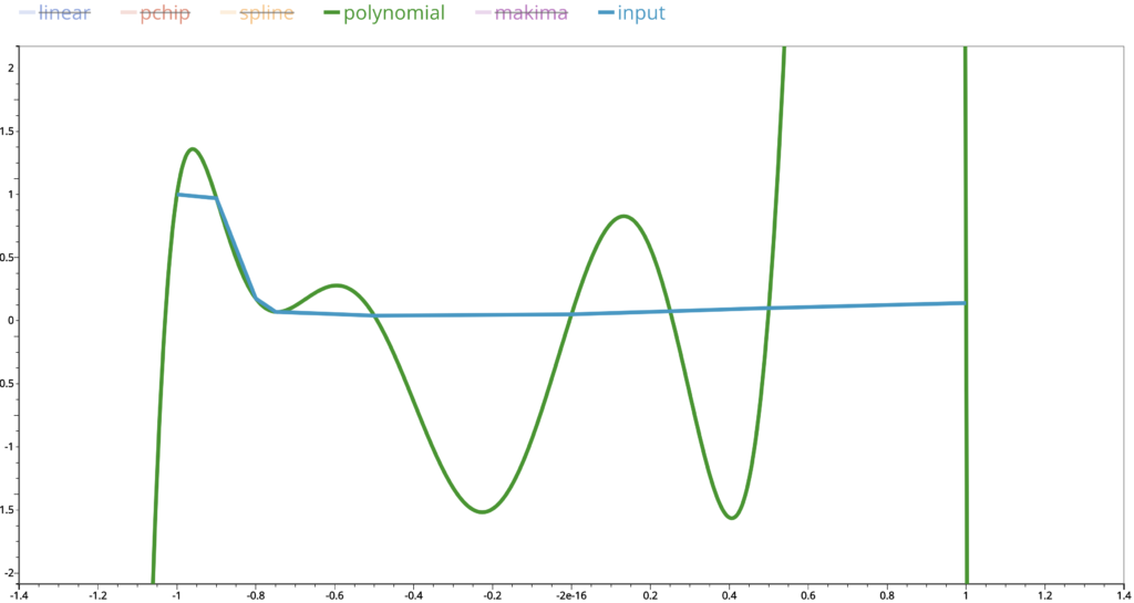
Even we ignore that part and zoom in more closely, we can see that there are still big up and downs in the interpolated values. This is similar for cubic spline interpolations.
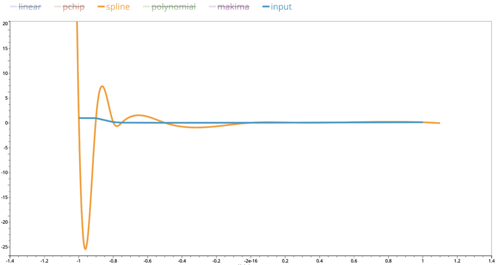
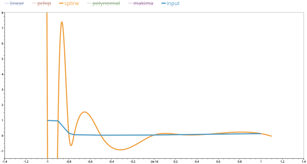
Remember that polynomial interpolation gives a polynomial function whose derivative functions of any order are continuous and cubic spline interpolation polynomial has continuous first and second derivative functions. These discrepancies are the price we pay in exchange of our pursuit of high level of smoothness in the interpolated curves.
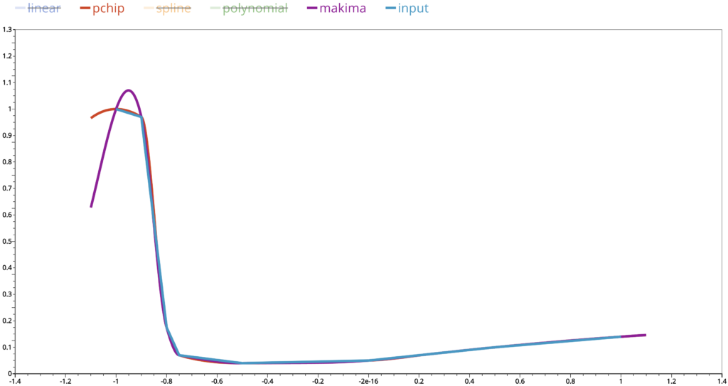
On the other hand, pchip output almost aligns perfectly with the linear interpolated curve. This is determined by the way it chooses the polynomial functions on each subinterval. It forces the interpolated values to stay close to the linear interpolated values. Makima is similar to pchip. Compared to pchip, some interpolated values are further apart from the linear interpolated values, but not as much as those from the spline or polynomial interpolation. We can consider it as a compromise between the cubic spline and pchip.
Interpolation application
We have seen how interpolation helps us to get a big picture based on limited data we have at hand. With the power to know the value at any location, we can use it in various scenarios. For example, when we want to multiply two curves, the two curves need to share common X values. What if the two curves don’t? We can provide a list of X values and perform a linear interpolation to both curves. As a result, the output curves will share the same X values. Since interpolated curve always passes through input points, it is guaranteed that no information will be lost as long as all the X values from both curves are included. If we can afford little information loss, we can tidy up the X values.
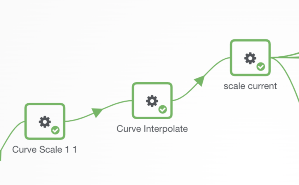
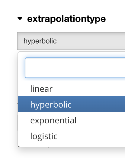
Interpolation worker helps us to understand the data within the range. When we want to obtain information outside the range of our data, we need to perform extrapolation. d3VIEW also have an extrapolation worker to help us. There are a few different methods available. Similar to interpolation worker, extrapolation worker can help us in a number of scenarios too.


