In the previous post, we have discussed about how interpolation works in general and reviewed a few commonly used interpolation methods. All these methods only consider the adjacent a few points. This works fine most of the time. However, in reality, data points further away from the interpolation point may also have some impact on its value. The scale of the impact though depends on the distance to the interpolation point. Usually, points further away contribute less than those close-by points.

Kriging is one of such interpolation methods that considers distance to the point during the process of interpolation. Not only it considers the distance, it also accounts for the correlation among these points. If we don’t consider correlation, contribution from two points that are very close may be overestimated.
Based on distance and their correlations, Kriging assigns different weights for each point and calculates the weighted sum to interpolate the value at the interested location.
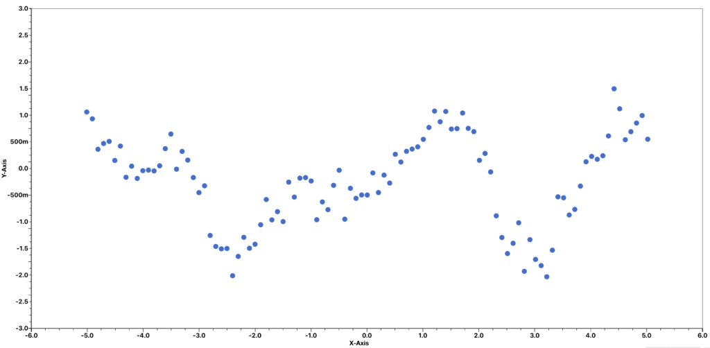
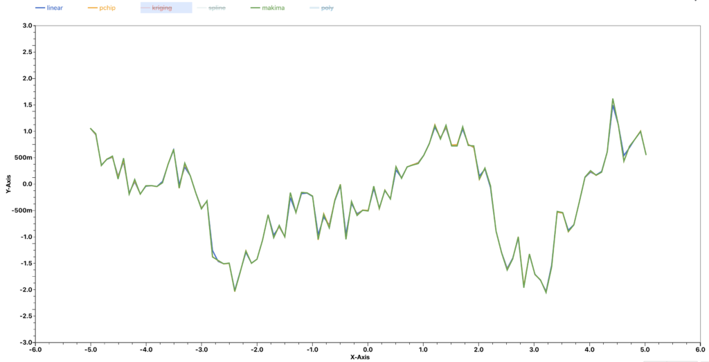
For example, when we are given a data set like this, we expect that many interpolation methods will generate a lot of zigzag patterns in the interpolated curve.
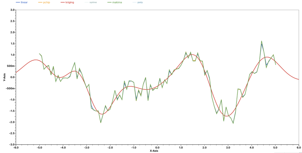
For Kriging, we can get an interpolated curve that is more smooth without these zigzag patterns with a small cost. The cost is that the interpolated curve will not cross all the given points. But the output curve still gives a close approximation and sufficiently describes the relationship between the two variables.
Kriging interpolation can be easily extended to higher dimension data too. Consider the following data.
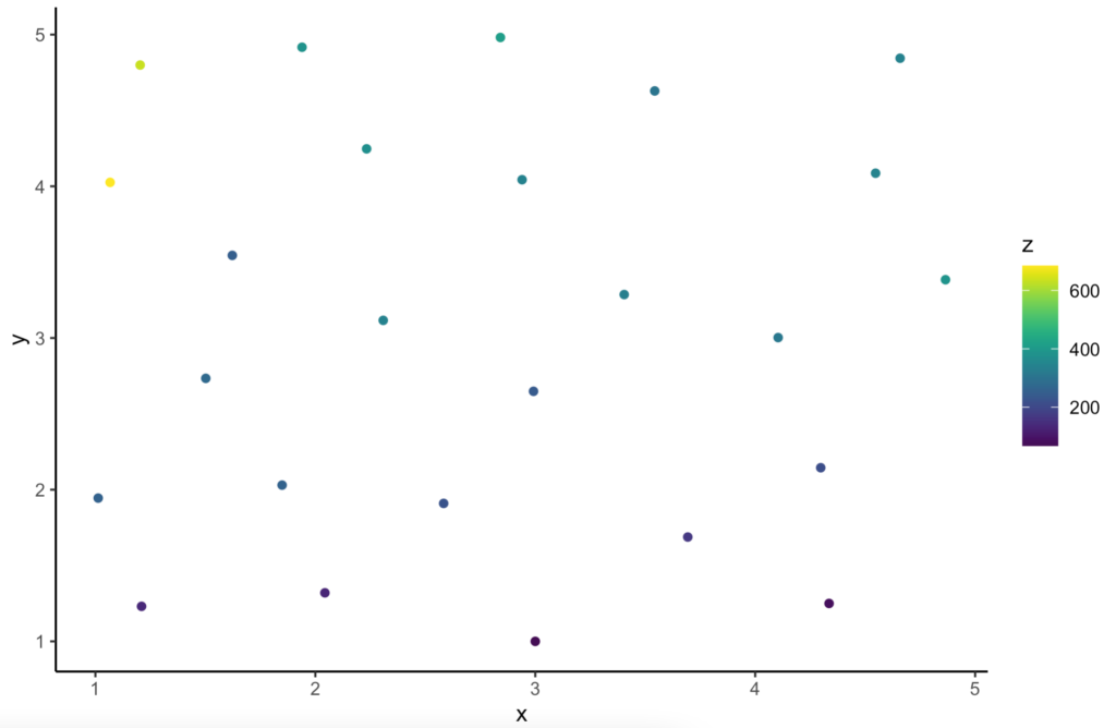
And the interpolated output on a 2 dimensional grid looks like this.
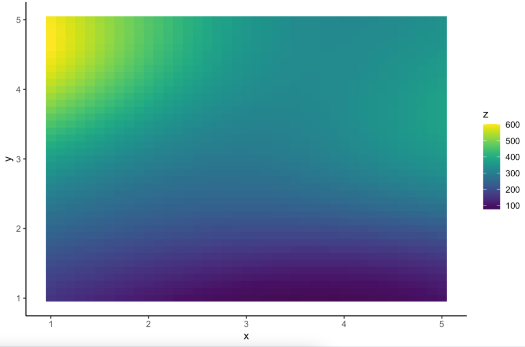
Overall, if the data points don’t have any correlation, then Kriging interpolation does not necessarily give better output. But in cases when we know there are correlations among points, Kriging interpolation can provide a more accurate results.


