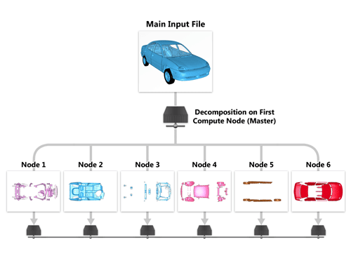
In the area of distributed computing using Massively Parrallel Processing (MPP) LS-DYNA, finite element model decomposition is performed after initial processing of the input deck to “distribute” the model content to compute nodes. There are two primary goals for model decomposition. First goal is of of course to “break-down” the given problem into smaller pieces based on the number of processors assigned. LS-DYNA writes the broken down pieces of the model in the form of a structured input file (scrXXXX) that will be reinitialized by respective compute nodes. This is shown in the following figure:

(Click image to enlarge)

The second goal is to provide a “equal” model sizes to each of the compute nodes to ensure a good load balance. The second goal of providing “equal” model content to all compute nodes is both dependent on the type of decomposition methods used and also on some internal logic built-into LS-DYNA. The type of decomposition can be specified in the ‘pfile’ (invoked at the commandline arguments) OR it can using the keyword *CONTROL_MPP_DECOMPOSITION in the input deck. LS-DYNA provides four different types of model decomposition. The default is the recursive-coordinate-bisection which recursively bisects the model about a plane perpendicular to the longest dimension. The initial model dimension along each global axis is computed based on the nodal coordinates (abs(Xmax-Xmin), abs(Ymax-Ymin), abs(Zmax-Zmin)) to give Xlen, Ylen, Zlen. After each ‘bisection’ these lengths are re-computed for each segmented model in a recursive fashion until the number of segmented model equals the number of processors. The initial longest dimension computed based on the nodal coordinate can be scaled to override the default dimensions. Decomposed model can be visualized (using LS-PREPOST) to understand the segmented models delivered to each processor using either the PFILE (show) or *CONTROL_MPP_DECOMPOSITION_SHOW in the input file. An example of specifying the decomposition method, scale-factors, and the option to dump the decomposed model is shown below:

Using Pfile
decomposition {
method rcb
sx 1000
sy 2000
show
}


Using Keyword
*KEYWORD
*CONTROL_MPP_DECOMPOSITION_METHOD
RCB
*CONTROL_MPP_DECOMPOSITION_TRANSFORMATION
SX,1000
SY,2000
*NODE
...
*ELEMENT
...
*END


Need for Scaling Dimensions in RCB Method
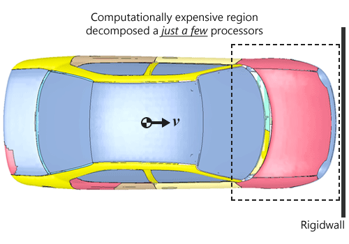
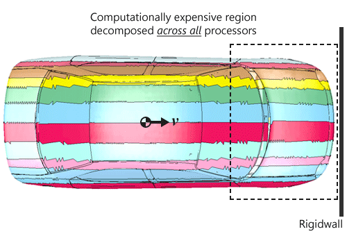
The option to scale the initial dimensions of the model is usually done to improve the load balancing and is entirely based on problem. In automotive simulations involving full-car crash events such as front-impact where an automotive is impacting a rigid-wall, most of the deformations and contact-impact are centered around the front-most portion of the automobile. Unfortunately, for RCB method, the original initial longest dimensions almost always happen to be along the impact direction, unless we start making automobiles that is wider than its length. This causes the recursive bisection method to split the model as shown in Figure 1 which results in a few processors having to deal with a lot of expensive computations which leads to improver load balancing where the remaining processors tend to have more idle time. In such cases, the user can easily scale the initial Y-LEN such that it becomes the most dominant length, and recursively bi-section this, will result in a decomposition shown in Figure 2 which helps in all processors sharing the more computational aspect of the model. Both figures 1 and 2 were generated using LS-PREPOST by reading the file “d3plot” file written by MPP-LSDYNA using the show command in the pfile or the *CONTROL_MPP_DECOMPOSITION_SHOW keyword in the input file.

Auto Scaling of Initial Dimensions
MPP-LSDYNA provides an option to auto-scale the XLEN, YLEN, ZLEN that is based on the logic of first determining the velocity vector. This logic is mainly implemented for automobile crash simulations which may apply to other areas. The logic works by first computing the initial dimensions and performing a check to see if its direction matches the initial velocity/motion vector defined using *INITIAL_VELOCITY,*CHANGE_VELOCITY and *BOUNDARY_PRESCRIBED_MOTION keyword. If they match, then the matching axis dimension is scaled down to a very small number. While this option helps to eliminate the need to know the scaling direction, it is always recommended to verify the segmented model.

Improving Load Balancing for Contact Definitions
Computations involving contacts in LS-DYNA usually take a 20-40% of total computational cost of most simulation models. Better load balancing and reducing communications can significantly improve the scalability and turnaround time of the models run using MPP-SDYNA. To improve load balancing, contact definitions must be equally distributed to all processors. This is usually done for contacts having large number of slave/master nodes/segments. To reduce communication between processors, smaller contacts needs to be isolated to individual processors. Both of these can be achieved using *CONTROL_MPP keyword. To distribute large contact definitions, the keyword *CONTROL_MPP_DECOMPOSITION_CONTACT_DISTRIBUE (or sdist in pfile) can be defined to specify a list of up to 5 contacts. To isolate smaller contacts, the keyword *CONTROL_MPP_DECOMPOSITION_CONTACT_ISOLOATE (or silist in pfile) can be defined to specify a list of up to 5 contacts to be isolated to certain processors.

Region Based RCB Decomposition
Starting from 971 revision 3 , LS-DYNA now allows a new way of decomposing a model which allows more flexibility in how the model can be segregated. Conceptually, it allows a sequence of unlimited number of regions to be defined which are then sequentially processed in the order of definition. A region can be defined as a logical combination of a box, sphere, cylinder, and/or a list of known part IDs. Each region can use its own scaling and transformation values. By default, each region is distributed to all processors and optionally, they can be lumped to just one processor. Region based decomposition is ideal for models whose global decomposition options result in poor load balancing. Consider a full-vehicle model with detailed occupant modeling for both the passenger and the driver. The global decomposition options with user defined transformation values provide no option to distinguish the treatment of occupants and in some cases could just lump the occupants onto just one or few nodes. Using region based decomposition, the occupants can be defined as a region and then be first distributed to all processors and then the left-over vehicle can be use the global decomposition values based on the load case. For a full vehicle front-impact analysis, the following region based definitions illustrates use of “region” keyword in the pfile.

decomposition {
method rcb
# occupant 1
region box xmin xmax ymin ymax zmin zmax sx 0.1 sy 1000
# occupant 2
region parts 1 2 3 4 5 6 .... sx 0.1 sy 10000
# global values for left-over parts (vehicle)
sx 0.1
sy 10000
}

Assuring Consistency and Accuracy of Simulation Results
While it is always good to use non-default decomposition methods and its options to improve load balancing and reduce communication overhead, it must be noted that using different decomposition parameters between design studies may cause variation in results. The testing of various decomposition methods and parameter must be done very early to choose the optimum parameters for a given run and these parameters must be fixed for the entire duration of the design cycle.