Similar to the dataset_simulated_annealing_optimizer worker, which takes a dataset as input, we can consider the curve_simulated_annealing_optimizer worker. It takes a curve as input and returns the optimal y value of the curve as output.

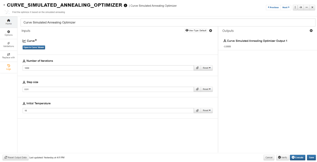
A curve can be considered as a dataset with two columns with each representing one coordinate of the points on a curve. The difference between the curve worker and the dataset worker is the way the model is built. With a curve input, curve interpolation techniques are used to find the values on a new location of the curve.

Example

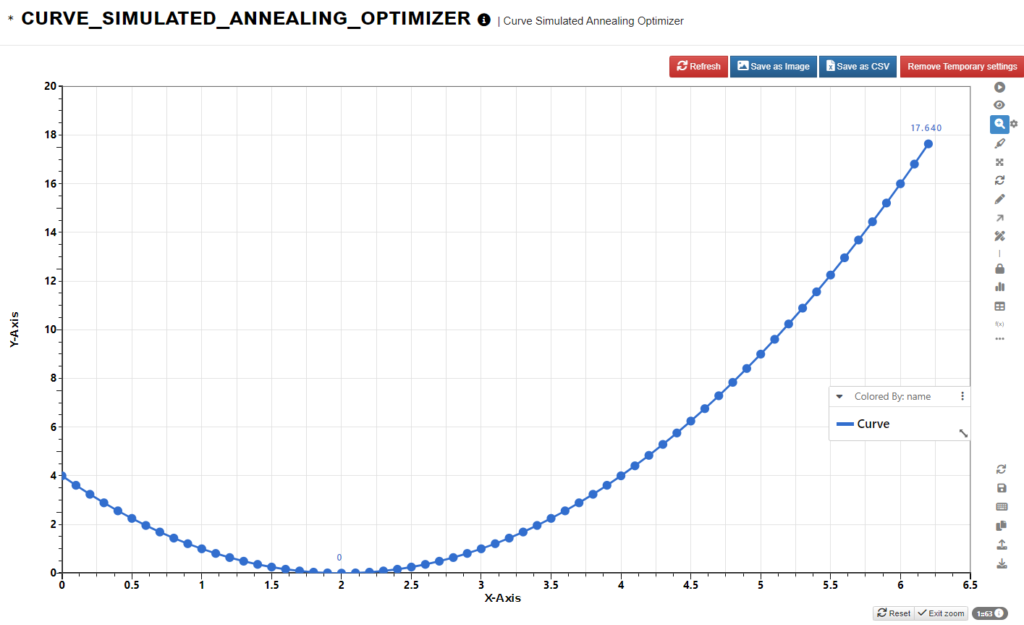
Starting with a parabola curve y = (x-2)^2, we know that the optimum is 0. Upload the curve to the worker input and execute the worker, we see the output is 0 as expected.

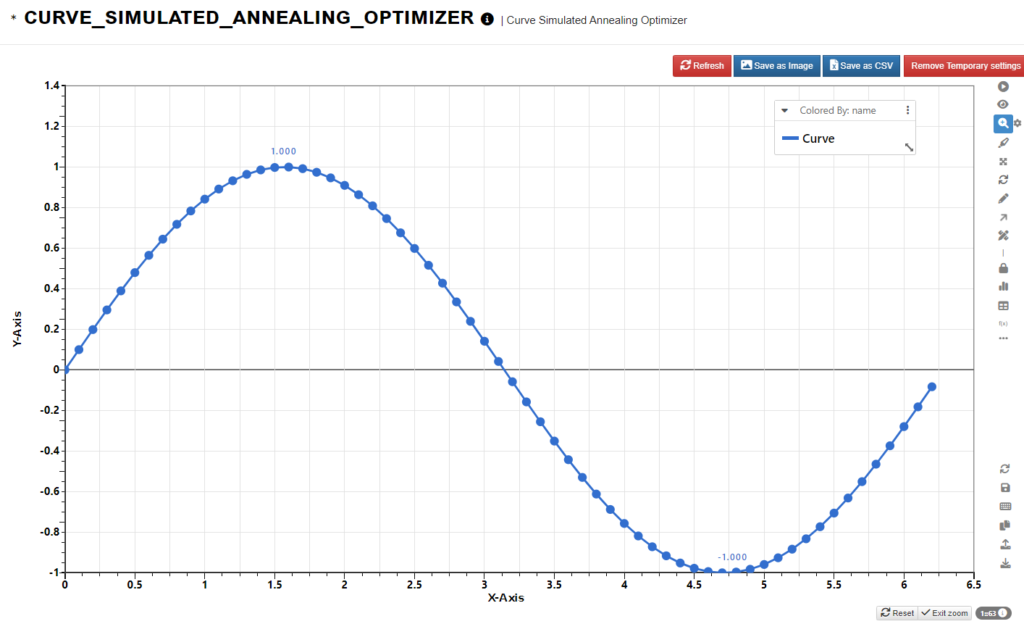
Replace the curve input by a sine curve that ranges from 0 to 2*pi (about 6.28). From experience, we know the optimum is at x = 5*PI/4 (about 3.927) with a min value of -1.

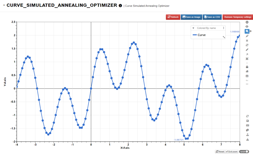
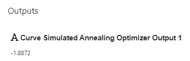
Now we can try a more complex curve with multiple local minimums. As we can see from the graph, the minimum is around x = 5 and the optimal value is about -1.88. Again, after running the worker, we get the expected output.