Curves are used widely to define a XY data that are used by several entities in LS-DYNA. They help us to define either a time-dependent function, used in loads and boundary conditions, and/or a strain/strain-rate dependent function used frequently in constitutive models. Three most salient features of curve representation, that occur internally in LS-DYNA and which is not quite obvious to the user, is the process of ‘digitization’, ‘extrapolation’ and ‘interpolation’. In this post, the internal extrapolation is addressed.
Need for curve extrapolation
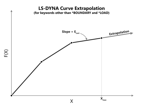
All curve inputs to LS-DYNA have a minimum and a maximum independent variable which we can label them as Xmin and Xmax that defines the independent variable range. During the simulation, when the instantaneous value of the independent variable, Xi, goes beyond this range, internal curve extrapolation, using the last available slope, is performed automatically by LS-DYNA as shown in the curve below. This is required as it is always not possible to anticipate the range of the independent values during the course of the simulation time frame and LS-DYNA helps us by doing the extrapolation to get the appropriate dependent values.
Extrapolation in Curves used by Constitutive Models
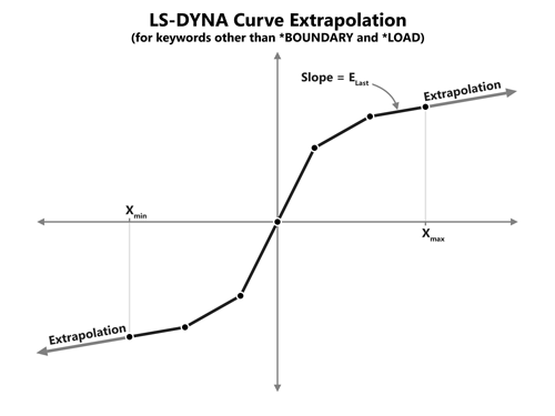
Most constitutive models use the curve input to allow the definition of the the stress/force as a function of the independent variable which could be strain/displacement. In many cases, uses input the values from the test data which may not necessarily provide the data to cover the entire range of the strain or displacement which necessitates the curve extrapolation. There are several situations where extrapolation is used and they are showed in the following figure.
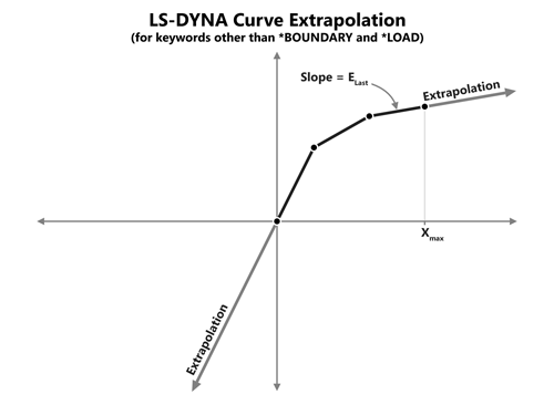
In the case of constitutive models used by springs and discrete beams, care must be taken to define a curve such that it passes the origin (0,0) to model the behavior in both tension and compression. If only one of the phase is defined, then LSDYNA performs extrapolation in the undefined phase using the last available slope nearest the origin in the defined phase as shown below.
Extrapolation in Curves used by Loading and Boundary Conditions.
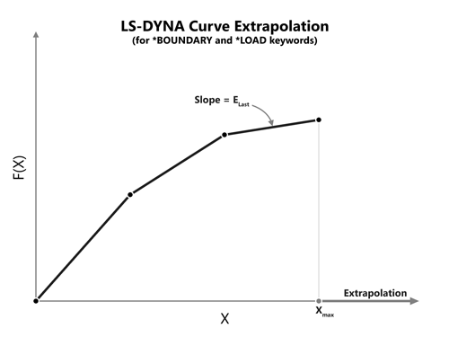
Keywords that define external loads such as *BOUNDARY and *LOAD skip the extrapolation and instead use a value of ‘0’ every time the instantaneous value of the independent variable, Xi, goes beyond the range of Xmin and Xmax as shown in the following figure. This is done to prevent the generation of non-physical forces due to the extrapolation based on the last available slope. It is therefore the user’s responsibility to ensure that last abscissa value is equal to or greater than the termination time of the simulation. This can be easily ensured by using a *PARAMETRIC_EXPRESSION in which the ENDTIM parameter in CONTROL_TERMINATION is first defined as a parameter variable and then using this as the last available abscissa point in all *DEFINE_CURVE keywords that are referenced by load type keywords. It is also possible to ensure a certain tolerance using the expression < &endtim+0.1*endtim> to extend the last available abscissa beyond the termination time which is necessary to avoid the movement of the nodes back to the initial coordinates when using the *BOUNDARY_PRESCRIBED_{option} keyword.
Exceptions to Curve Extrapolation
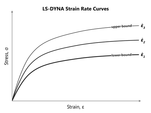
There is one important exception to the curve extrapolation when defining strain-rate dependent material model using DEFINE_TABLE keyword. To eliminate non-physical scaling of the yield surface, the yield surfaces that correspond to the lowest and highest strain-rates act as the bounds of the yield surface scaling such that the stresses do not exceed these bounds. This is shown in the following figure.


