Domain decomposition is central to MPP-LSDYNA as it determines the final load balance on each of the compute nodes. The default (and most widely used) decomposition method is the Recursive Coordinate Bisection (RCB) which recursively halves the model using the longest dimension of the input model.

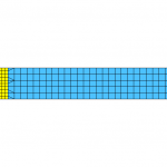
Halving the model along the longest computed length of the model may seem like a good choice but will eventually result in unequal portions of the models for a model with varying element count and element formulations. This leads into the question about how MPP-LSDYNA handles the weighting of the element count and the formulation. To demonstrate this, consider a simple plate which has a fine and a coarse mesh as shown below, run using 2-CPUs. In the first 2 cases, the element formulation chosen for both parts is the default “type 2” formulation and both parts use “ELASTIC” material law.

1. No weighting of element count
With no weighting with regards to element count and the formulation, the RCB method will use the longest dimension, which happens to be along the length of the plate (x-direction) which will result in the model divided along the center line yielding one processor getting a lot of elements while the other with a very few elements. A perfect load imbalance.

2. Weighting of element count
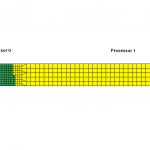
By default, MPP-LSDYNA first computes the longest dimension of the model (in our example it will be x-direction length) but it does not stop here. It continues to calculate the number of elements along this direction and moves the center line such that the final center line will result in the equal amount of elements after division. Using the “show” command in the “decomposition” section of the “pfile”, the resulting decomposed model is show below.

3. Weighting of element formulation
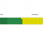
In this case, the coarse mesh element is now switched to “type 16” formulation which is roughly 3 times more expensive when compared to the default formulation. This non-uniform element formulation along the longest dimension determined by RCB is taken into consideration by MPP-LSDYNA which then again moves the centerline such that the elements are weighted against its formulation to give roughly provide element count that takes the same amount of computational cost. The decomposed model is shown below where you can see that it has moved the center line more towards the right even though the number of element count is more on Processor 0 since it is made of mostly inexpensive “type 2” elements.

4. Now what about out-of-plane (NIP) integration points ?
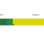
This is taken into account as well. In our example, the element formulation for both parts are now switched back to “type 2” but the coarser mesh now uses NIP=9 while the fine mesh uses the default value of NIP=2. The final decomposed model (shown below) is nicely divided to give roughly equally expensive element set.

5. What about the material cost of the element ?
To evaluate this, the coarser mesh was switched to MAT_024. The resulting decomposed model did not change since the material cost is not taken into account by MPP-LSDYNA as it has no knowledge about when the elements would undergo plasticity.

Thanks to Dr. Jason Wang of LSTC for sharing info on this internal logic.